Fit a truncated Functional Generalized Linear Model

Fit a truncated functional linear or logistic regression model using nested group lasso penalty. The solution path is computed efficiently using active set algorithm with warm start. Optimal tuning parameters (\(\lambda_s, \lambda_t\)) are chosen by Bayesian information criterion (BIC).

Usage

fglm_trunc(
  Y,
  X.curves,
  S = NULL,
  grid = NULL,
  family = c("gaussian", "binomial"),
  degree = 3,
  nbasis = NULL,
  knots = NULL,
  nlambda.s = 10,
  lambda.s.seq = NULL,
  precision = 1e-05,
  parallel = FALSE
)

Arguments

Y: n-by-1 vector of response. Each row is an observed scalar response, which is continous for family="gaussian" and binary (i.e. 0 and 1) for family="binomal".
X.curves: n-by-p matrix of functional predictors. Each row is an observation vector at p finite points on [0,T] for some T>0.
S: (optional) n-by-s matrix of scalar predictors. Binary variable should be coded as numeric rather than factor.
grid: A sequence of p points at which X is recorded, including both boundaries 0 and T. If not specified, an equally spaced sequence of length p between 0 and 1 will be used.
family: Choice of exponential family for the model. The function then uses corresponding canonical link function to fit model.
degree: Degree of the piecewise polynomial. Default 3 for cubic splines.
nbasis: Number of B-spline basis. If knots is unspecified, the function choose nbasis - degree - 1 internal knots at suitable quantiles of grid. If knots is specified, the value of nbasis will be ignored.
knots: k internal breakpoints that define that spline.
nlambda.s: (optional) Length of sequence of smoothing regularization parameters. Default 10.
lambda.s.seq: (optional) Sequence of smoothing regularization parameters.
precision: (optional) Error tolerance of the optimization. Default 1e-5.
parallel: (optional) If TRUE, use parallel foreach to fit each value of lambda.s.seq. Must register parallel before hand, such as doMC or others.

Value

A list with components:

grid: The grid sequence used.
knots: The knots sequence used.
degree: The degree of the piecewise polynomial used.
eta.0: Estimate of B-spline coefficients \(\eta\) without truncation penalty.
beta.0: Estimate of functional parameter \(\beta\) without truncation penalty.
eta.truncated: Estimate of B-spline coefficients \(\eta\) with truncation penalty.
beta.truncated: Estimate of functional parameter \(\beta\) with truncation penalty.
lambda.s0: Optimal smoothing regularization parameter without truncation chosen by GCV.
lambda.s: Optimal smoothing regularization parameter with truncation chosen by BIC.
lambda.t: Optimal truncation regularization parameter chosen by BIC.
trunc.point: Truncation point \(\delta\) where \(\beta(t)\) = 0 for \(t \ge \delta\).
alpha: Intercept (and coefficients of scalar predictors if used) of truncated model.
scalar.pred: Logical variable indicating whether any scalar predictor was used.

Details

Details on spline estimator

For an order q B-splines (q = degree + 1 since an intercept is used) with k internal knots 0 < t_1 <...< t_k < T, the number of B-spline basis equals q + k. Without truncation (\(\lambda\)_t=0), the function returns smoothing estimate that is equivalent to the method of Cardot and Sarda (2005), and optimal smoothing parameter is chosen by Generalized Cross Validation (GCV).

Details on `family`

The model can work with Gaussian or Bernoulli responses. If family="gaussian", identity link is used. If family="binomial", logit link is used.

Details on scalar predictors

FGLMtrunc allows using scalar predictors together with functional predictors. If scalar predictors are used, their estimated coefficients are included in alpha form fitted model.

References

Xi Liu, Afshin A. Divani, and Alexander Petersen. "Truncated estimation in functional generalized linear regression models" (2022). Computational Statistics & Data Analysis.

Hervé Cardot and Pacal Sarda. "Estimation in generalized linear models for functional data via penalized likelihood" (2005). Journal of Multivariate Analysis.

Examples

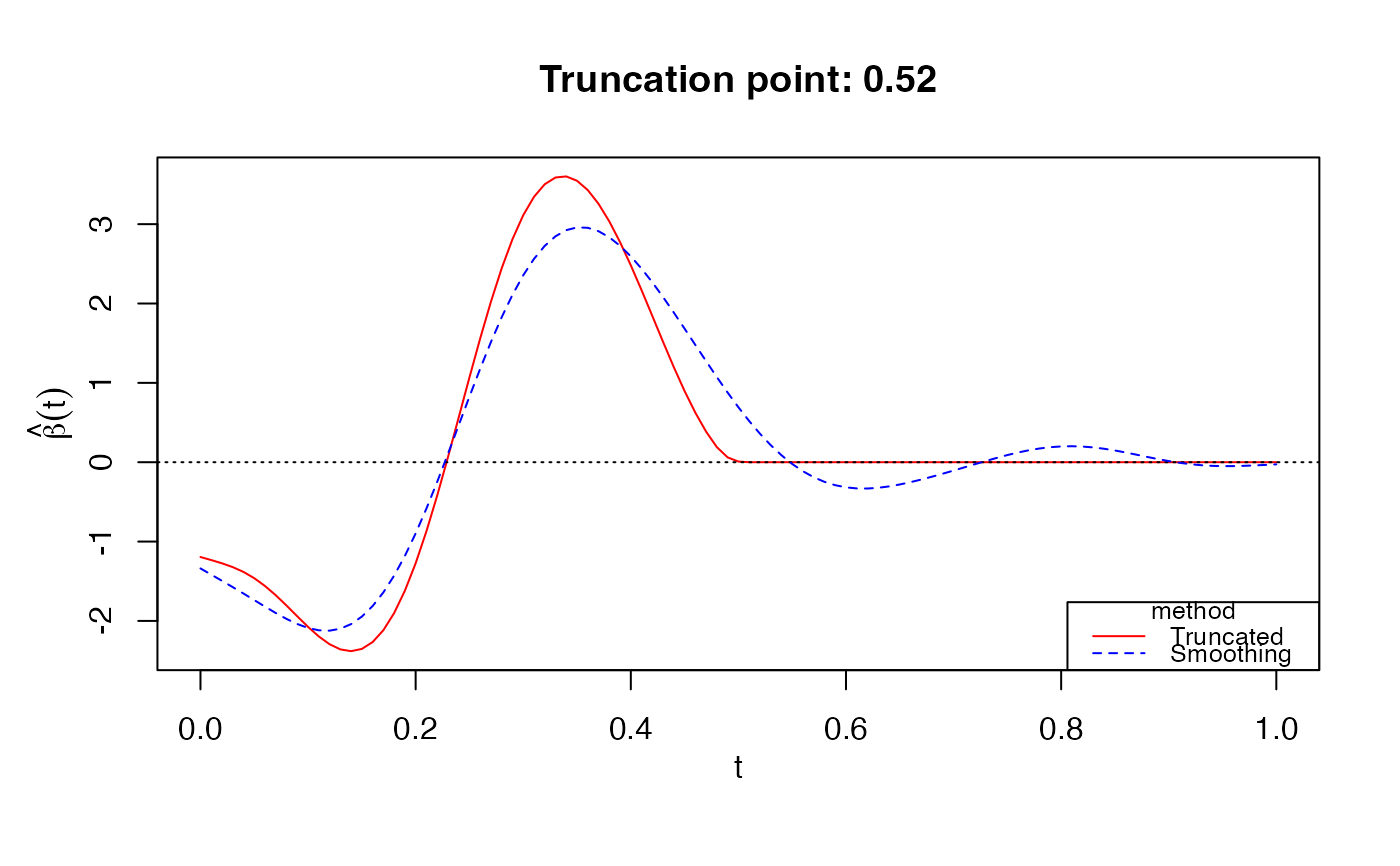
# Gaussian response
data(LinearExample)
Y_linear = LinearExample$Y
Xcurves_linear = LinearExample$X.curves
fit1 = fglm_trunc(Y_linear, Xcurves_linear, nbasis = 50)
print(fit1)
#> 
#> Call:  fglm_trunc(Y = Y_linear, X.curves = Xcurves_linear, nbasis = 50) 
#> 
#> 
#> Optimal truncation point: 0.52 
plot(fit1)


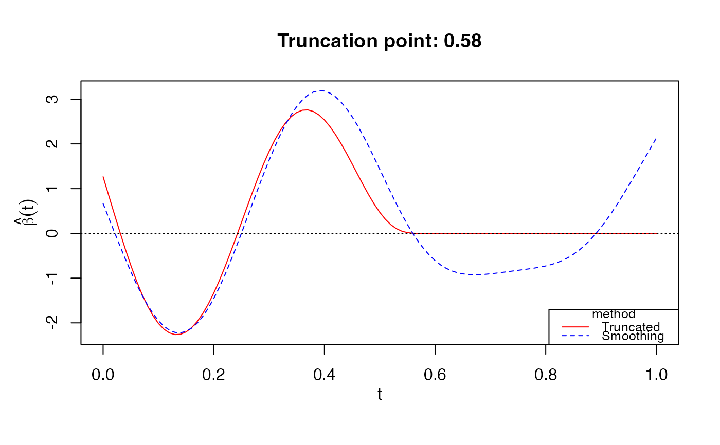
# Bernoulli response
data(LogisticExample)
Y_logistic = LogisticExample$Y
Xcurves_logistic = LogisticExample$X.curves
fit2 = fglm_trunc(Y_logistic, Xcurves_logistic, family="binomial", nbasis = 50)
print(fit2)
#> 
#> Call:  fglm_trunc(Y = Y_logistic, X.curves = Xcurves_logistic, family = "binomial", nbasis = 50) 
#> 
#> 
#> Optimal truncation point: 0.58 
plot(fit2)


# Parallel (NOT RUN)
# require(doMC)
# registerDoMC(cores = 4)
# fit3 = fglm_trunc(Y_linear, Xcurves_linear, nbasis = 50, parallel = TRUE)